An Overview Paper Being Offered to the Editor-in-Chief of
Elsevier's Journal of Petroleum Science & Engineering
for Peer Review and Possible Publication.
By Walter Rose
(edited on 12/5/2003)
Table of Contents
ABSTRACT
key words
INTRODUCTION
Background Ideas
DISCUSSION
Ad-hoc Theory for Simple Systems
Formulating More Complicated Cases
‘Unfinished’ Capillary Imbibition Algorithms
CONCLUDING REMARKS
NOTATIONS
AKNOWLEDGEMENT
REFERENCES
APPENDICES ADDED IN PROOF
1. Equation Road Map
2. Ad-Hoc Algorithms
ABSTRACT
The content of the watershed paper of Buckley & Leverett (1942)6 is being revisited here to further resolve some algorithm formulation difficulties examined by the present Author some 15 years ago (1988)19. Questions long-overdue are addressed again about the possibility of further upgrading the basic classical Buckley/Leverett Algorithms so that their use will better yield intended trustworthy predictions of future reservoir states. In a nutshell, our simple aim here is to search for practical ways to facilitate the monitoring of certain types of petroleum recovery transport processes. Specifically, these occurrences are ones that typically transpire during production of oil from subsurface reservoirs which exist as scattered local features associated with many worldwide regional aquifers. In particular, we shall be justifying our ideas by considering plausible transport process models that can show how (and better yet also show why) entering reservoir upstream formation and/or injected waters can efficiently displace and replace in-situ pore space oil ganglia so that they coalesce and move naturally towards the downstream production wells.
According to the classical ways of thinking, however, the proof that rationally-based reservoir performance algorithms are being employed is adequately confirmed when eventually definitive field and laboratory experiments have been undertaken. And these are the ones where the measured experimental output data turn out to be good history-matching predictors of actual subsequently observed field performance events.
This logical way to proceed is illustrated in what follows by focusing on somewhat simplified but representative reservoir cases. Here, for example, we start by dealing with an attempt to rationally model certain idealized irreversible two-fluid phase flow transport processes. Specifically we have in mind ones where wetting liquids like brines spontaneously happen (say, because of prevailing ambient artesian conditions) to replace and displace into production wells a portion of the non-wetting oil phase fluids that originally were present in the pore space of particular petroleum reservoirs. These are events that occur in reservoir systems such as those found in stratigraphically bounded sand lenses and/or in distributed up-structure entrapments like anticlines.
The classical approach to deal with these kinds of occurrences is: (a) To first postulate the applicability of a plausible theory based on what can be identified as modified Buckley-Leverett dogmatic ideas4,6,8,10,12.19; and then (b) To confirm whether or not the data obtained in subsequently scaled physical model (and/or Gedanken) experiments appear to be sufficiently supportive of the selected theory. Thereafter, it then becomes a job for reservoir engineers and their managers to guard against accepting any surprising non sequitur ambiguities that seem to surface if and when contradicting laboratory model data are obtained.
Lastly, we call attention20-30 to what seems to be new in our present 'revisiting' of earlier advocated algorithmic presumptions, which include: (a) Our reemphasizing of the advantages coming from adopting coupled rather than traditional Darcian flux-force relationships so that irreversibility effects are better taken into consideration; and (b) Our willingness to favor the use of computational algorithms that stochastically yield good forecasting information even when the theoretical justifications remain obscure.
Key Words: Idealized Petroleum Reservoirs; Transport Process Models; Simplistic Buckley-Leverett Algorithms; Viscous Coupling Effects; Anisotropic Media Properties; Capillary Imbibition Fluxes and Forces.
INTRODUCTION
We start by recalling that in 1988 an overdue attempt was made19 to upgrade and extend the usefulness of what were only popular vintage Buckley-Leverett algorithms2,8.10,31. Unlike Patek's recent 'revisiting' style (2002)13 to confirm the correctness of the content of the original 1855 Fick paper on "Liquid Diffusion", our approach here has been to focus on simple (but not necessarily fully tested) plausibly rational approaches, and even on grossly simplified ones26.31, whereby at least partial proof of the applicability of some of them could be prospectively accepted and applied in practical ways for the modeling of coupled multiphase porous media transport processes. This means, of course, that verbalizations of generalized rules must be concocted that take into account how modern ideas about coupling phenomena control various representative transport process outcomes of general interest12-23. In particular, it is this kind of information that is wanted to facilitate the modeling (and hence the accurate forecasting) of future field production outcomes that arise because of the underlying causative nature of the transport processes that are assumed to be involved.
Under consideration here to provide background for the topics to be discussed are the ideas expressed in six key monographs3,4,5.8.11.12, and also in a lot of the here cited (but perhaps less-read journal papers by the present Author. These citations in turn further point to a vast collection of scattered international papers which in turn likely point to other documentation of special interest to curious readers.
However, while many perplexing and disputed issues still remain unresolved even after the elapse of more than a half Century following the publication of the cited 1942 watershed B/L paper6, only some of them have been critiqued persuasively enough to earn general acceptance. Accordingly, it should not be expected that what written on these pages will conclusively settle all remaining issues of disagreement.
The fact of the matter is that the full proof of either the original or the modern-day opinions about the viability of underlying Darcian-based Buckley & Leverett dogmatic presumptions actually can not be fully assessed until coherent experimental proofs of at least some of the many postulated, practiced, and published contentions have been fully confirmed. What will be found in the following text, therefor are mostly suggestions of new ways to significantly rephrase some of the questions that can be asked today about those innocent positions taken in bygone times. In particular, upon accepting the preamble statements that appear in the cited Rose (1988) paper19, our modest aim now is simply to verbally offer without full proof some alternative analytically-appearing algorithms. And we take this approach as being a prospective Cartesian way for future workers (particularly the modern experimentally-minded modern ones) to improve and perhaps confirm the use of what seems to be acceptable alternative ad-hoc ways of thinking. And indeed that is why in what follows we prospectively choose to imply as our principal thesis that strictly linear models perhaps adequately describe many two-phase, isothermal. and low-intensity flows of immiscible Newtonian fluid pairs in homogeneous, isotropic, consolidated, water-wet porous rock samples that are perturbed because of superimposed viscous coupling and superimposed spontaneous capillary imbibition effects.
Background Ideas: As in the earlier Rose (1988)19 paper, we start by affirming the relevance of the nicely phrased conservation of mass statement by Buckley and Leverett, but reject their Darcy-based statements because of the arguments given by Rose (1999)25 and Rose (2000)27. But where Buckley & Leverett6 left matters ruminating now for more than 60 years, and indeed where many contemporary scholars like Hadad et al10 in one way, and Siddique & Lake (1992)31 in another also continue to do so, remains justified as an interesting but perplexing question of mostly passing historical interest.
In any case, and indeed without apology, we accept the sense of the Buckley-Leverett mass conservation theorem as phrased in Equations (1) to (4) below, but as will be seen, we categorically adopt the modern viewpoint due to enlightened thinkers pioneered by DeGroot and Mazur (1962) 7 that proper flux-force relationships to describe entropy-producing coupled (hence irreversible) transport processes so far have not so far been indicated by experiment to be Darcian in character as originally was (and in some quarters still is) wishfully presumed.
Eqn. Box 1
In Equations (1), for example, it is indicated that we are prepared to be dealing (say in a finite element mode) with transport due to capillary and gravity as well as to mechanical forces acting in three-dimensional space, where fluxes of mass/energy laden fluid particles and displacements occur (as Tribus32 uniquely mentioned a long time ago).
Figure 1, for example, is a not-to-scale schematic cartoon depicting how transport is thought to occur, for example in two-phase petroleum reservoir systems that are imbedded in regional aquifers. Depicted there are upstream t container rock system 3.o downstream pore network domains with source and sink termini to topographically complex in-series and parallel interconnected pore paths. These in turn lie within contiguous macroscopic representative volume elements (so-called RVEs) occupied spaces which in total constitute the porous medium reservoir system space that is made up of the fluid-filled interstices which both surround and are surrounded by 4 the solid mineral-occupied constituents of the container rock system network.
Figure 1
Specifically, what is wanted, of course, are laboratory ways to test whether the transport process theory that is under consideration can be authenticated by examining the data obtained in scaled model physical experiments. For example, here we shall be advocating the use of Rose's (1997)24 recently described laboratory methodology that appears conceptually and uniquely to be well-suited for the intended data-gathering purposes (e.g. as described in Appendix 2). Before further emphasizing this critically important contention, however, we choose first to introduce the idea that the ad hoc transport process theory to be considered here is made evident by the sense of the following algorithmic formulations that appear in the 19 Equation Boxes that are scattered throughout this paper (and also further referenced in Appendix 1). As will be seen, verbally the major cited equations assert that: (a) Whenever and wherever low intensity diffusive fluxes are involved, linearity between conjugate fluxes and forces are to be expected. This supposition, for example, is elegantly suggested by Bear (1972, cf. §4.4)3; and (b) Even so, simple mathematical relations and clever laboratory measurement methodologies likely (and luckily) also seem to be involved that avoid the need to search for and employ possibly non-existent reciprocity relationships between either the diagonal or cross transport coefficients that otherwise might be wanted in order to facilitate determining values for them from the experimental data.
Equations (1) and (2) above, for example, are phrased to facilitate focusing on ad hoc ways to describe certain both steady- and unsteady-state petroleum reservoir transport processes. The example selected ones are those which are clearly based on mass and/or energy conservation principles. Particular attention will be limited for simplicity to important cases where the reservoir pore space domains at all times are represented as being completely saturated by two essentially incompressible and immiscible Newtonian liquids such as: (a) in situ connate water together with any injected or otherwise invading aqueous liquid phases; and (b) any previously unproduced original oil-in-place. Each of the selected RVE macroscopic domains of the representative reservoir depicted in the paper's Figure 1 will be chosen also for simplicity to be characterized by possessing locally constant porosity magnitudes that can be predetermined. Moreover, the parameter subscripts {1,2}={W,N} for the process variables are employed simply to make it clear which fluid phase will be found when and where during thc course of the ensuing reservoir transport processes. Thereby, appearing in those relationships (viz where the local positive or negative accumulations of each of the two fluids are being referenced) the first term on the left-hand side of Equations (1) will be seen to be exactly equal to the 'inflow minus outflow' convergence's of the designated fluid phases as expressed by the second left-hand term of the same Equations. Hence Equation (2) shows that the sum of the companion two fluid phase flux divergences locally will be exactly equal to zero.
Accordingly, that is why Equation (3) then indicates that the local time-changing flow transport processes under consideration are ones that involve vector operations like addition gradients, multiplication of vectors by scalars, scalar and vector products of two vectors, gradients and divergences of scalar and vector fields, and the Laplacian of scalar and vector fields as deal with compactly by the Bird et al (2002)5 classic text on Transport Phenomena.
In these connections, notice that the adjacent ganglia of wetting and nonwetting fluids as seen at the pore level frame-of-reference in general will display curved (locally convex or concave) interfaces in turn have both stationary and moving microscopic curved fluid-fluid interfaces. And the topology of the angle of approach they make along the lines where wetting and nonwetting fluid elements approach the surface of the bounding solid pore space walls is such that indicates that implies that prevailing capillary driving forces also may contribute to the local convergences and associated divergences of the two companion fluid phases. In any case (3) shows that when flow transport locally is to some extent directed in non-horizontal directions, this means in consequence that the superimposed gravity forces cannot safely be ignored (N.B. see Tribus (1961, p. 520 ff.)32. Finally, with respect to Equation (4), when the transport processes under study are ones where so-called capillary pressure gradients can be ignored, we have the result that: Eqn. Box 2
![]()
Here the two Equations (1a) are intended to describe low-intensity uncoupled 2-phase fluid flow in isotropic media as though Darcy's Law holds for two phase systems, and as such they are equivalent to Equations (20a) in the text. Also clearly for the following Equations (1a) necessarily to be derivatives of the first ones so far have not been proven experimentally … but only innocently presumed by some early and later workers according to Rose14-18,25,27 as well as by other investigators from Yuster to those mostly modern workers (for example, as cited in the body of this paper36,33,34,36,37).
In passing, however, it is also very much worth noting that Equations (1a) as they stand can also be employed to describe low intensity flow of single phase Newtonian fluids in two-dimensional anisotropic media under conditions shown in a recent Letter to the Editor of Transport in Porous Media by Rose (1996) 24b.
To continue our analysis of how to upgrade and modernize traditional Buckley-Leverett ways of thinking, we look at Equations (5) and (6) shown below as polynomials where the coefficients of linear proportionality are those dozen somewhat redundant and symmetrically interrelated saturation-dependent terms that appear in Equations (7). These as seen to express the not unexpected and logically plausible linear transport relationships that seem to properly model why and how the causative thermostatic and thermodynamic forces give rise to the consequent fluxes and displacements by which natural non-equilibrium systems irreversibly approach final end states.
Eqn. Box 3
In passing. we notice that both Equations (5) and (6) display flux versus force relationships for two water-oil fluid phase saturated systems that however are written in two inherently equivalent ways for cases where only a single coupling type (e.g. like viscous coupling) is involved. These two disparate equation forms are: (a) Either where the fluxes are shown to be expressed with three terms on the equation right-hand side (i.e. where the transport coefficients appear as upper case Latin letter notations like [A,B,C,….]); or (b) More commonly, compactly and usefully with only two terms on the equation right-hand side (i.e. where the transport coefficients appear as lower case Greek letters notations like [α,β,γ, …]). Equations (7), and then (7a) below then show the simple mathematical relationships and notational equivalencies between the six Greek and six Latin letter transport coefficients. And, as seen in both (5) and (6) transport equations for each fluid, the simple coupled transport processes involve the same two identical driving force terms as shown below in Equations (5a,6a) as written below in matrix form. These latter Equations will be seen to apply to cases where the pore space is saturated with two immiscible fluids, and where only a single type of coupling has to be considered, and that involves two fluxes and conjugate forces. And so we write:
Eqn. Box 4
Clearly, to monitor and numerically describe the steady and unsteady states of the transport processes which are called for by Equations (1) above, we start with the above two equations given in the (5a,5b) matrix form which independently provide relationships since the various Dij are independently given as functions of saturation are experimentally observable and simply measured in terms of the available flux-force data. Implicitly then, two additional independent relationships will be needed that also explicitly relate the Dij to other laboratory experimentally obtained flux and conjugate force data. Then with the four Dij relationships all known and established, values for the {Ω,Ψ) terms as functions of saturation can be inserted in Equations (1) to generate the wanted relevant forecasts of steady and unsteady state segments of anticipated future reservoir process events.
Implied more generally, for example by Equations (7), is that with the superscript (ω=1.2.3.4), we can then designate the four semi-redundant experiments that can be performed in order to compute values for the 12 overlapping transport coefficients from the measured values of the conjugate flux/forces pairs, (Jr,Xr) where {r,s}={1,2}. Specifically, this possibility can be seen in the interpretation of Equations (8) below which presents in matrix form the senses of Equations (5) and (6) when applied to the several distinct experimental cases. For example, in the first experiment, both driving forces are non-zero and also not equal to each other. In the second and third experiments one of the driving forces is set identically equal to zero, but the other one not. And in the fourth experiment the two driving forces are equal to each other. And this means in effect that we have eight independent relationships which are sufficient by the method of simultaneous equations to extract numerical values for the two sets of six transport coefficients of proportionality as identified by Greek and Latin characters in Equations (7). And, remarkably as a special feature of the unique experimental method being employed 9.24.35, the capillary pressure (and hence the local saturation) can be held fixed and constant during the course of the course of the ensuing suites of the four experiments to be conducted at each system saturation level (and this even though the Jr fluxes and displacements and Xs measured force data values will tend to be differ during the conduct of each experiment type.
Eqn. Box 5
Here it is seen that the first two of Equations (8) are to be conducted by observing the 1 and 2 fluxes by imposing the two driving forces to be unequal with each other and not equal to zero. Then in the second and third sets of experiment first one and then the other driving force is set equal to zero, while in he fourth experiment the two driving forces are constrained to be equal to each other nor equal to zero. Other independent sets of experiment could be ones where the companion travel direction cold be set to be counter-linear rather than collinear.
DISCUSSION
In these connections and as alert readers can carefully note, the Rose reference in (1997)24 shows explicitly how for two-phase (say water-oil) liquid saturated porous rock, a novel laboratory procedure is made available by the unique instrumentation characteristics of an apparatus system by which the validity and utility of the computerization algorithm that is chosen for various specified applications.
We are now ready to address the fact that to forecast what happens when a horizontally oriented anticline reservoir that has been more-or-less lying dormant over long periods of geologic time (i.e. before eventually they are first accessed contemporaneously) by systems of special upstream and downstream injection and production wells. These are both to provide entry for the displacing aqueous fluids, and to permit commercial lifting of available oil to the surface collecting facilities such as separators, gathering and distribution pipelines, refinery process installations, storage tanks, waste disposal facilities, and the like. Here as we consider the petroleum recovery process, we now will be assuming that it in part will be at least approximately modeled by idealized relationships such as the first two of Equations (8). To proceed, however, we must cope with the problem associated with the fact that for the present case now under consideration where there are two transported entities (i.e. n = 2), and where implicitly we will need two more independent relationships so that with Equations (8) we now will be dealing with four then. It is then that by solving 4 by 4 matrix simultaneously that we can thereby extract values for the needed four Dik transport coefficients.
Ad-hoc Theory for Simple Systems: As it turns out, Aitken (1956, Chapter II)1 describes (as did other authorities both in antiquity and in modern times) the classical ways to solve independent simultaneous equations which while conceptually straight-forward is occasionally computationally complex. Accordingly, we abandon here employing the popular method of determinants, but more simply consider the ideas developed in the recent disclosure of Rose and Robinson (2004, in press)30. And we do this first for the particular case presently being considered for illustrative purposes, namely where we start out only having two governing equations with four unknowns, but then are left dealing with the need to find the equivalent of two other independent relationships so the four equations can be solved simultaneously.
Specifically, by arranging for the two driving forces in two successive experiments to alternately and sequentially have the values implied by the four line vectors shown on the left-hand side of Equation (9a), then the four Equations (9b) to (9e) and the four Equation (9f) clearly follow, or: Eqn. Box 6
In other words, Equations (9a) can serve as the four relationships necessary to solve for the four transport coefficients in terms of experimental measurements. These are seen to be calculated from the experimentally measured force to flux ratios that are the saturation dependent parameters as Equations (9b) to (9i) indicate. Specifically all of Equations (9) represent the form which the parent Equations (1) and (2) in Box 1 will have for the particular n = 2 case under discussion.
Below in Figure 2 copied with permission from the indicated Rose (1997)24 TiPM paper, schematically shows how the measurements called for by the Equation (9) algorithms actually can be made. Proof of this contention as given below also implicitly follows from considering the experimental methodology described earlier in the works by Dullien & Dong (1996)9, and before that by Zarcone & Lenormard (1994)35, , and indeed before that when Rose (1976, cf. Appendix)17 was organizing a petroleum engineering curriculum at the Institute of Technology at Nigeria's University Ibadan.
The Figure 2 apparatus arrangement which has been referenced in a number of the Author's recent publications24.,25,27.28,29,,38,39 is also further critiqued in Appendix 2 of this paper.
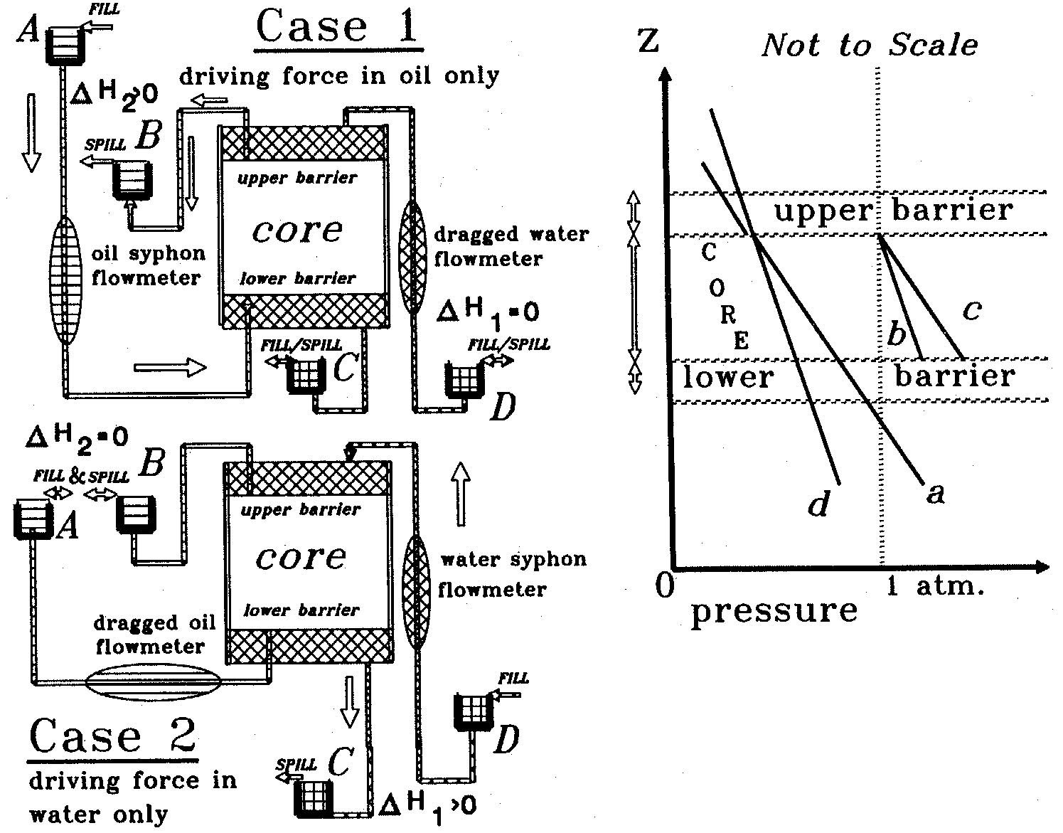
Figure 2 - (After Rose in TiPM, 28: 221-231 (1997)24
A proper legend for Figure 2 implies the following. Here are schematic depictions of Case 1 and Case 2 scenarios shown in the left-hand diagrams, respectively, for where in Case 1 the imposed gravity free-fall driving force is proportional to the difference in elevation of the free surfaces of the non-wetting fluid contained in the A and B siphon reservoirs where {(ρ2 g H2) = X2 } > 0, whilst the imposed driving force in the wetting fluid contained in the C and D siphon reservoirs is zero since {(ρ1 g H1) = X1} = 0. Similarly, during the second set of experiments, then in the Case 2 experiments the imposed gravity free-fall driving force is zero in the non-wetting fluid since in the A and B siphon reservoirs it is {(ρ2 g H2) = X2 } = 0, whilst the driving force imposed by the elevation difference of the wetting fluid contained in the C and D reservoirs is finite since it now follows that {(ρ1 g H1)=X1 } > 0.
In these connections, notice that for the Case 1 experiments, the oil is being pushed up by an amount indicated by the oil siphon flow meter because A is always kept filled while the excess oil is spilled from the B reservoir. And the water also is dragged upwards by the viscous coupling effect since C is kept filled and D spills at the rate indicated by the dragged water flow-meter. And then opposite things happen during the Case 2 experiments because the water is pushed down at a rate indicated by the water siphon flow meter since the level in D is greater than that in C, while the oil is dragged down by the viscous coupling effect at a rate measured by the dragged oil flow meter because the A and B oil fluid levels are kept at the same levels.
Clearly, the following Equations (10) relationships, formulated specifically to apply for manipulating the data obtained when conducting flow experiments for the two ingenious Cases 1 and 2 configurations illustrated on the right-hand side of Figure 2. These, as seen, are consistent with indications of the earlier general relations already anticipated by Equations (1) and (2). Here we notice that the two fluxes in general will be given by the sum of the pushed portion caused by the imposition of an imposed driving force plus the dragged portion caused by the viscous coupling effect. In other words, we have:
Eqn. Box 7
To be noted in passing, Equations (10) also apply to the laboratory configuration for the measurement scheme illustrated in Figure 2. The latter has been purposely designed so that operationally in the successive experiments that first one and then the other driving force terms are set equal to zero. In such cases, the only finite external driving force that remains is that provided by the gravity drainage action of a siphon which results in the companion force to be positive-definite. In fact, it is this unique configuration arrangement which makes it possible during each set of the successive experimental episodes, to have two phase flows occur where the capillary pressure gradients (and hence the associated saturation gradients) re,arkably are identically zero during the steady-state two-phase flow episodes. Hence we now can accept Equations (11a) and (11b) as shown below. Hence for the Case 2 Formulae we have:
Eqn. Box 8
And for the Case 1 Formulae we have:
Eqn. Box 9
To be noted here is the interesting fact that redundantly the validity of the above relationships to some degree can be obtained by equating the first of Equations (11a) to the last of Equations (11b), and likewise by equating the last of (11a) to the first (11b). And more than that, by forming a ratio between the second of (11a) to the second of (11b), one can assess whether or not the Phenomenological Equations of Onsager (cf. as given by DeGroot & Mazur7) asserting that (Dij = Dji) perhaps may or may not apply for the particular transport processes being characterized by Equations (9) and (10).
Formulating More Complicated Cases: Finally, we close the overview discussion by employing the ideas of Rose and Robinson (2004, in press)30, and also the related ideas to some extent already illustrated in other recent publications28,29. And as above in the previous subsection to this paper, we extend our discussion of rationales for on occasion employing generalized ad hoc (rather than fully justified empirically and theoretically based algorithms) as sensibly accurate and economic ways to easily model even more complicated cases of coupled irreversible fluid phase transport processes. These in fact are those important ones which are known to commonly occur in porous sediments.
The ones under consideration, however, do not seem to correspond except perhaps superficially to those other important special-case processes like thermo-diffusion which have been described by the followers of Onsager with such acuity by DeGroot & Mazur (1962)7 and many others by invoking the Principle of Microscopic Reversibility.
In these connections, it will be remembered that when one has in mind representative volume elements (i.e. RVEs) viewed as continuums in which multiphase transport processes are occurring, then from the Eulerian point of view one may think of them as fixed averaged spatial locations where extensive system quantities in unsteady-state processes are seen to be changing with time. Alternately, from the Lagrangian point of view, one may think of such RVE locations as being occupied by a ‘droplet-train’ succession of traveling fluid particles (following one after the other along tortuous streamline paths) where each one contains a fixed amount of some extensive quantity of the mass/energy phase under consideration. And then there may be various associated state variables that happen to be aboard and dragged along with the moving fluid particles.
Specifically, the macroscopically observable motions seem to occur due to the action of prevailing mechanical and/or internal energy driving force energy gradients. Analytical expressions for these motions are given below as Equations (12a) and (12b) in the form previously presented by Rose (1995)25 for particular miscellaneous transport process of interest. Thus we hazard to suggest that the situation being monitored:
Eqn. Box 10
![]()
It is in Equations (12a) where the summation rule applies, that we find ourselves now considering what we are calling ad-hoc relationships that interestingly enough are superficially similar in appearance to the early afore-mentioned classical Onsager relationships. For example, in coupled thermo-diffusion systems the α,β superscripts stand for thermal and chemical energy fluxes, but in Equations (12a) they can stand for the {W,N} terms that designate the two-phase immiscible wetting and non-wetting pore fluid phases … while the {x,y} subscripts stand for the Cartesian two-dimensional spatial locations.
On the other hand, the ambiguous (12b) formulation clearly lacks the definiteness of the classical Onsager Reciprocity Relationships. Accordingly, we find ourselves now left facing the heretofore somewhat neglected task of inventing and authenticating what amounts to plausible intuitively-based rationalizations for these relationships.
Anyhow, as a way to facilitate and expedite our search for closure to the nagging questions about how to model the dynamics of questionably non-diffusive transport process cases, we now can jump to considering the interesting but severely complicated cases of two-phase isothermal flow of single component and incompressible fluids in anisotropic media systems whenever viscous coupling effects in addition are a prominent feature to be considered.
According
to the cited Rose (1995)25 paper, the above Equations
(12a) display with a simplified notation the possibly probable linear
relations between fluxes and forces which are predicted if and when
the indications of Equations (12a) are to be believed to apply to the
case of 2-phase flow in 2D anisotropic media. And Equations (13b)
which appears below seem to indicate plausible symmetry relationships
that may be cautiously applied if needed. But to be trusted they must
be verified by experiment. In
such a case, for example, in Equations (12b), Rose (1995)23
and (1996)38
has suggested that relationships displayed by the sixteen
![]() transport coefficients of (12a) might in some cases experimentally
prove to be:
transport coefficients of (12a) might in some cases experimentally
prove to be:
<![]()
![]() >
>
![]()
![]() >
>![]() where
where
![]() >?<
>?<![]()
![]()
The equivalence of them, however, to the sixteen Dijαβ diffusive flux transport coefficients given in Equations\ Boxes 7 to 13 [i.e. where Equations (11) to (15) ae located] at this point so far has not been established, hence the existence of reciprocal relations between the terms of Equation (13b) remains as an open question, but not one necessary to be addressed here. As will be seen, this is because of the ease with which other independent relationships can be formulated to render the necessary matrix relationships determinant.
Upon expanding Equations (12) we can write Equations (13) as:
Eqn. Box 11
![]()
Here Equations (13a) present four scalar equations containing 16 initially unknown transport coefficients, and Equations (13b) show in the classical manner how at least 12 independent definitions for the non-diagonal ones provided enough additional relationships so that the matrix problem becomes unambiguously determined, and this without the need to verify in advance which (if any) of the reciprocity relationships postulated (by the (13c) and (13d) relationships need to be experimentally verified.
For example, we may consider an innovative device presented by Rose (1976)18 and revisited again in (2001a,b)28,29, to uncover more than 16 independent polynomial equations where the elements of the defining matrix can be defined in terms of knowable laboratory measured functions of the corresponding scalar elements of the observed flux and force vectors. The proof of this is in fact supplied by the formulated in Rose and Robinson (2004)30 in ways described below and again in the Appendices that follow.
To close this particular discussion, we may briefly illustrate the obvious fact that the application of Equations (12) and (13) can be extended to other more simple as well as more complicated cases of non-diffusive transport processes. One of these is case of two phase viscous-coupling affected flow in isotropic media where we seek by the methods of determinants to obtain expressions for the four transport coefficients for this case. And we shall show this can be done without the need to a priori presume the existence of symmetry conditions.
For the two phase cases we shall be dealing with, in order to simplify to simplify the argument, wee adopt the symbolic notation for the flux, force and coefficient terns which are employed below, or:
Eqn. Box 12
![]()
![]()

As shown by the Equations (14), two independent experiments are performed by letting the driving forces alternately be set first at some finite measured value and thereafter set equal to zero as indicated by noting that Equations (9d) and (9e) together provide four equations for calculating the four unknown {A,B,E,F} transport coefficients from the flux and force measured data. The paper of Rose (1997)24 describes a measurement methodology by which the required number of experiments to be conducted can be suitably performed.
For readers who think it is a waste of time to conduct so many complicated experiments to measure the transport coefficients needed to conduct computerized simulations of particular reservoir transport processes, it is the opinion of this writer to caution that it is a false economy to try to minimize the expenditure of laboratory time and expense when the consequence is that only flawed misinformation will be the result! And the same is true, or course, when trying to save computer time and expense by employing less costly computational algorithms which are an insidious guaranteed to obtain faulty calculations.
‘Unfinished’ Capillary Imbibition Algorithms: Finally we consider it to be a matter of great importance to call attention to the formulation of viable algorithms which in a rational way can be predictors of what we descriptively call forced versus spontaneous capillary imbibition reservoir processes. There are at least four interconnected reasons why this should be true, as follows: (a) Involved in many (if fact almost all cases of ordinary reservoir usage's) immiscible multiphase fluid phases are seen and caused to flow variously out of, through, and/or into the pore space of subsurface reservoir rock domains; (b) The associated transport processes which are involved are comparatively complex and not well understood in terms of the microscopic quantum laws that only loosely can be employed to explain observed macroscopic behavior; (c) The fact is that almost all oil and gas subsurface accumulations co-exist with and/or are contiguous to bottom and edge water aquifers influxes, and sometimes also to injected surface waters; and (d) These displacements and replacements often are subject to the complex and often dominant action of important capillary forces that affect the movement of the resident subsurface hydrocarbon fluids.
One reason to deal with what to many is a perplexing capillary imbibition subject matter is because of the fact that quite frequently various petroleum recovery process cases are encountered that involve the replacement of hydrocarbon fluids with initially resident or invading aqueous phase ganglia that become entrained in bounded subsurface sedimentary pore space. This is a subject not only touched on below as an 'unfinished' (meaning not well-understood) topic of commercial as qwell as scientific importance, but also one worth revisiting by reading in Appendix 2 to follow how the topic needs unraveling and unscrambling and extrication before reservoir engineers of the 21st ebtury can say that the art of constructing truly coherent algoritmic forecasts of petroleum reservoir behavior. For example, the ordinary water-flooding process after-all is a paradigm example affirming the relevancy of developing clear understandings about this subject now being discussed. Here, however, it is to be agreed that the formulation of coherent reservoir simulation algorithms involves complications that heretofore have not always been widely or wisely treated.
For example, one class of difficulties has to do with the fact that sometimes it is the inherent complexity of the attending transport process coupling effects that must be taken into account. These arise because of the dual way the invading aqueous phases in general can be caused by mechanical and/or as well as by free surface energy driving forces. The latter is where the former are imposed and/or imparted because of accompanying fluid injection processes, while the latter are the consequence of inherent capillary actions that automatically give rise to spontaneous imbibition of the wetting fluid.
Accordingly, herein an effort is made to deal with the attending problems of describing the complex nature of the commonplace petroleum recovery processes where inbibition in one form or another occurs. In particular, three general cases therefore will be at least partially considered, namely: (a) Where the attending driving forces alone involve mechanical energy gradients acting on the bulk fluid phase elements; (b) Where in addition, there are also free surface energy gradient driving forces existing, and this because of local wetting phase saturation variations in time and space that give rise to spontaneous capillary imbibition effects; and (c) Where no resulting saturation gradients that are finite in magnitude exist within the pore space domains being investigated, and this even when steady-state conditions are finally reached.
Some 30 years ago it was Jacob Bear (1972)3 who was the earliest one of several later monograph authors like Marle (1982)12, Bear & Bachmat (1990)4, and Dullein (1992)8 who took the trouble to recognize that Yuster's 1951 watershed paper34 provided a foundation upon which certain rational analytical algorithms modeling non-equilibrium coupled transport processes involving diffusive fluxes possibly could logically be based on Onsager's famous 1931 Reciprocity Relationships for which a Nobel Prize finally was finally awarded in 1968 (cf. Rose in 196915). Here, however, for the non-diffusive cases currently being considered, only a few minor amplifications of the general theory can be informatively restated here. This is because the relevancy of that subject matter for capillary imbibition applications so far is by no means fully established. The intention as mentioned in previously given commentary is to follow economical ways to increase practical understandings about the oil field applications, rather than to get overly immersed in considering obtuse second-order theoretical matters.
In other words, the intention of what is being written now is to modestly uncover further clarifications that still are needed so that the ideas being dealt with in current works can more fruitfully be employed by investigators who are engaged in reservoir simulation studies of hybrid spontaneous versus induced capillary imbibition and related coupled processes.
Specifically to be dealt with in what follows here is the nature of the transport processes that commonly occur in porous sediments when saturated by pairs of immiscible fluids for those common cases where one of them usually can be considered to preferentially ‘wet’, hence adhere to the pore space surfaces more strongly than any other of the contiguous immiscible fluid phases. And in our analysis, but with only minor loss of generality, the fluids can be idealized as being homogeneous, chemically inert, incompressible, and possessing a Newtonian rheology. Furthermore, the porous medium for its part will be taken to be uniform, usually isotropic, rigid, insoluble, and chemically non-reactive. Finally, and for simplicity, attention will be limited to isothermal transport processes of low intensity (viz. so the fluid flows will be laminar in character). And the underlying theme of the remarks to be made below quite naturally will deal with the perplexing question about why so many past and present authors in general have seemed to think that spontaneous capillary imbibition effects can be treated as though they are caused exclusively by the action of mechanical energy driving forces even for cases where common sense alone makes it clear that such processes inherently are the result of the action of free surface energy gradient driving forces.
The description of the transport processes of the two-phase systems as to be described here, for example, already was first given in an approximate way by the Author in two of his recent disclosures (cf. Rose 2001a,b) which are both based on a timely revisiting of an earlier Sabbatical Leave (1963)28a paper by W. Rose here cited in two current papers28,29. The canonical forms appear in Equation Boxes 13 and 14 a Equations (15) and (16) which apply to the general case of where there may be two fluid flow fluxes and/or one parallel and accompanying free surface energy flux. These presumed nondiffusive fluxes, for example were shown to be driven respectively by two conjugate mechanical energy gradient forces, but also occasionally by an associated and superimposed free surface energy gradient force term as discussed previously in an enlightened way by Tribus (1961)32. Thus we have:
Eqn. Box 13
and also:
Eqn. Box 14
In the above Equations (15) and (16), the subscripts, {i,j} = {1,2} respectively designate the wetting (say W = aqueous) and the non-wetting (say N = hydrocarbon) pore fluids; hence the Ji are the so-called Darcian approach velocity vectors for the two fluids which are locally at measurable pore space saturation levels, Si, and where respectively the Xj for {j =1,2} are the conjugate mechanical energy gradients (per unit mass) acting as forces to give rise to the ensuing two phase flow processes. Note that these are shown above to be identically equal as the intended way to achieve a quasi-zero zero dynamic capillary pressure gradient … and hence a uniform (or at least a steady-state saturation condition) during the flow measurements (cf. Rose, 1997)24. On the other hand, these equations XE and JE respectively, refer to free surface energy gradient driving forces and fluxes which are manifested by spontaneous capillary driving force effects of those special sorts perceptively mentioned by Tribus (1961)32 where he draws a distinction between how non-equilibrium thermostatic and thermodynamic processes should be separately considered.
For example, in Equations (16) notice is to be taken of the fact that in total there are nine transport coefficients, Dij , which each are functions of how geometrically the pore space of the sediment is partitioned throughout time and space between the two locally present immiscible fluid phases. Clearly experiments will have to be performed to establish the quantitative form of these linear dependencies. Moreover, for starters there are the three flux-force relationships and the three Onsager Reciprocity Relationships that are given by Equations (16). Also notice should be taken of the fact that in the experimental work to be performed, imposed values of the mechanical energy gradient driving forces, XW and XN, can be selected such as those shown in the right-hand matrices of Equations (17) for what are being illustrated as the logically chosen four separate experimental measurement cases that need to be performed. And, in passing it is to be also noticed that the fluid flux terms, JW and JN are ones that easily can be measured with conventional flow meter instrumentation for each of the four (A,B,C,D) laboratory test cases.
Specifically, in Equations (15) or (16) there are admittedly a large number of independent, dependent and disposable variables to be dealt with.. And what is to be sought are a similar number of independent relationships to evaluate their characteristic variations with respect to time and position. Logically, four separate steady-state experiments with the same ambient saturation values and interstitial saturations distributions locally are to be held constant for each of them, as indicated by the chosen decision to separately undertake the experiments prescribed by the four sets of Equations (17) as being the logical ones to be performed. This choice, of course, is so that numerical values can be obtained for the transport coefficients as explicit functions of saturation, spatial location and temporal time during the ensuing recovery--processes.
Eqn. Box 15
Accordingly, Equations (17) above have been presented in order to identify the flux-force conditions that apply to the four {A,B,C,D} cases of separately independently undertaken experiments. The objective of this experimental approach, of course, is so that with Equations (18a,b,c) as also given below, a display can be given for the three dependent and six independent (Dij ) material response transport coefficients that can be assessed from the given input values of [Xi ={,β,γ}] together with the observed values of the [Ji ={1,2, and sometimes 3}] measured flux data.
The problem of combining the Equations above that are presented in order to obtain useable coupled capillary imbibition algorithms, however, clearly lies in the fact that the J3 and X3 terms which refer to the spontaneous capillary imbibition flux and driving force parameters sometimes will not be as clearly observable and/or easily and directly measurable as the are in the slightly different cases where the multiphase flow caused by mechanical energy gradients is coupled with unambiguous concentration and/or temperature gradient forces which give rise to heat and mass transfer effects.
For example, however, by manipulating with the terms of Equations (17), auxiliary useful relationships can be developed such as:
Eqn. Box 16
In Equations (18a), the flux terms that are wanted are the nine (j=αβγJi=1,2,3). And these essentially the ones that themselves are not directly measured during the (A,B,C,D) experimental tests. That is, it is mainly the (i = 1,2) flux elements that can be easily observed for these (A,B,C,D) experimental tests since each of the (A,B,C,D) fluxes are summations involve a somewhat un-measurable ±γJi flux terms caused by the ± γ driving forces.
Combining Equations (17) with (18a), then one can easily obtain definitions for all of the transport coefficients, as:
Eqn.
Box 17
The matrix Equations (18b), of course, define how the {A,B,C,D} experiments provide the data needed to calculate the values in space and time for the nine material response transport coefficients, Dij, that is by dividing line-by-line the elements of the left-hand flux matrix by the corresponding directly measurable force elements of the right-hand matrix. Thus even for cases where γ is finite in magnitude (hence giving rise to possible spontaneous imbibition effects), we have the ratio values for the non-zero Dij elements of the central matrix of Equations (18c), such as:
Eqn. Box 18
and so forth. In these connections, however, it must be mentioned in fairness that the indicated values for the ambiguous diffusivity element, D33 shown in the ninth position of the third column of the central matrix, is perhaps questionable, but unfortunately at the present time no other clever way so far has been discovered to remove this uncertainty except by observing real-time experimental data.
To summarize the senses of what has just been described above, notice can be taken of the agreeable fact that by sequentially (but separately) performing the four {A,B,C,D} experiments defined by Equations (17), but for the desired result to be obtained, of course. this must be done in a way where reference values for the local fluid phase saturation's and interstitial saturation distributions are held fixed and constant until all of the four experiments have been performed in each sequence of interest. That is, the investigator will be obtaining laboratory data which when combined: [a] with input data about the three driving force terms, Xj where these will be X1 = α or zero; X2 = β or zero, and X3 = plus or minus γ always (1), and [b] with observational data about the two measurable flux terms, J1 and J2, then eventually the nine transport coefficient (material response) terms as defined by Equation (18b) and (18c) can be unambiguously computed either uniquely or even sometimes redundantly, as shown below. Thus, it follows that:
[1] By sdtarting with Experiment D, and by observing {DJ1 } and {DJ2 = - DJ1 } and by knowing gamma, γ, one can compute {D13 = D31 } and {D23 = D32 } (and/or also by making use of presumed analogs of the Onsager Reciprocity Relationships) as functions of Saturation and Saturation distribution. On the other hand, if one wishes to verify the applicability of the definition given in Equations (18) above as independently and explicitly providing a correct value for D33, one then must seek still other means to deduce and know values for the four {AJ3}, {BJ3 }, {C J3 }, {DJ3 ) terms.
[2] Then by performing Experiment A, and by observing {AJ1 and AJ2 } and applying the plausible reciprocity Relationships, and additionally by knowing the input magnitude of α one now can compute values for the { D11 } and {D21 = D12 } terms.
[3] Then by performing Experiment B, and by observing { BJ1 } and { BJ2 } and again applying the available reciprocity Relationships, and additionally by knowing the input magnitude of {α}, one now can finally compute redundantly the { D12 = D21} and the { D22 } term.
Eqn. Box 19
As previously shown elsewhere6,10,19,20,31, those who have and continue to adhere (blindly or otherwise) to Buckley-Leverett dogma, would say that for two phase flow where the driving forces are only mechanical energy gradients, it is clear that the following simple definitions for the Ψ and Ω parameters of Equation (19) that apply to the Darcian modeling case will be those that appear on top line of Equations (20), while those that apply to the coupling cases appear on the bottom line, as follows:
Eqn. Box 20
Clearly the algorithm on the first line of Equations (20) applies to outdated Buckley-Leverett assumptions dogma which have been discredited to some extent in certain current papers25,27,36,, while the algorithm on the second line is to be employed to take viscous coupling effects into account20 And Equations (21) below, however, are offered to ’fly’ in the face of those who are puzzled by the idea that has been proposed and questioned recently26,37 to the effect that spontaneous capillary imbibition perhaps can be the result of mechanical as well as surface energy driving forces! Thus, when with X3 > 0, the view is held here that when spontaneous capillary imbibition processes will be involved along with viscous coupling effects, that in this case then one should consider making use of the following more general finalrelationships:
Eqn. Box 21
To be noted in connection with Equations (21a) and (21b), however, is the important fact that spontaneous capillary imbibition effects can only occur in those domain regions of the system pore space where the X3 (Capillary Driving Forces) are of finite (i.e. non-zero) magnitude. Clearly, such a condition, of course, only holds whenever and wherever locally and for whatever reason the wetting phase saturation is changing with time. In contrary cases, the 3rd, 6th and 9th rows of the matrix Equations (18b) are eliminated and disappear, leaving the simplex Equations (20) rather than the complex Equations (21) to serve as the algorithms that will properly describe those partially unsteady-state processes dealt with earlier20 for cases where capillary driving forces are not involved because imposed conditions are such that finite saturation gradients are somehow everywhere avoided throughout time and space when the Dij terms are being measured by the laboratory procedures described and/or simply referenced by Rose24.
In conclusion, if a comparison were to be made between the early papers by the Author on the dynamics of capillary-controlled reservoir processes with those that have followed up to the present time , the reader might wonder why it has taken more than a half-Century for him to be now composing still another newly based one. The fact of the matter is that some writers tend to be thinking faster than they write while others engage in the opposite. Even so, the Author will find it reassuring if at least some of the reader of this paper agree that a rational algorithm to
model capillary imbibition processes necessarily must be one that will enable undertaking reservoir process simulations if and when the following propositions are found to be true. 5
If the displacement mechanisms under study are ones where viscous coupling or analogous effects may possibly occur, then this is reason enough to employ Equations (21) with Equations (1) as a safe way to formulate trustworthy ways to forecast future reservoir performance. More than that, if the displacement mechanisms are ones where spontaneous imbibition possibly is occurring, this will provide a second and even more compelling reason to employ the algorithm of Equations (21) over the simplistic ones imbedded in Equations (20) when reservoir simulation computations are being undertaken. But finally, if because of the possible intervention of burdensome time and cost factors, some still think that there are persuasive reasons to employ short-cut reservoir simulation methodologies, such ‘wishful thinkers’ should keep in mind that prudence alone may dictate that the value of these questionable ways of thinking must be proportional to the conclusions arrived at by conservatively undertaken parallel cost-to-benefit ratio assessments.
CONCLUDING REMARKS
(a) If the displacement mechanisms under study are ones where viscous coupling or analogous effects alone may possibly occur, then this is reason enough to employ Equations (20) as a precautionary way to formulate trustworthy ways to forecast future reservoir performance.
(b) If the displacement mechanisms are ones where spontaneous imbibition possibly is occurring, this will provide a second and even more compelling reason to employ the algorithm of Equations (21) in spite of incurring burdensome time and cost factor inconveniences , some still think that there are persuasive reasons to employ short-cut reservoir simulation methodologies, such ‘wishful thinkers’ should keep in mind that prudence alone may dictate that the value of these questionable ways of thinking must be proportional to the conclusions arrived at by conservatively undertaken parallel cost-to-benefit ratio assessments.
Finally. It is worth suggesting that negative as well as positive points of possible special interest to practical reservoir engineers might include the following:
(a) Exactly (it may be asked) how can one conduct experiments and obtain as many independent linear force-flux relationships as there are numbers of the initially unknown transport process coefficients of proportionality? This question clearly needs further quantitative study. After all, it is necessary to fully confirm the fact that the latter indeed can be unambiguously assessed by the standard simultaneous equation solving methodologies as applied to standard models of the various local transient saturation level changes that model the accompanying imbibition and drainage cycles that will be occurring. This complex matter will surely occupy the attention of future investigators.
(b) So far as whether a comprehensive theory for describing spontaneous capillary imbibition phenomena can ever be fully developed, a weakness is to be anticipated and acknowledged about the use of a simplistic capillary pressure gradient term for the driving force instead of a surface energy gradient term.
(c) With reference to the {α, β, γ, δ, ε, φ } composite transport coefficients of proportionality seen in the second of Equations (5) and (6), and related to the {A, B, C, D, E, F} transport coefficients as seen in Equation (7), and also the Dij related transport coefficient terms seen in Equations 9, 10 and 11 are consequences of the mind-boggling fact that it is implied that {α+β-ε}= 0 = {γ+δ-φ}! The deeper meanings of this curious result clearly needs further study.
(d) The point is to be emphasized that although the cost of conducting careful multiple experiments is high (and sometimes prohibitory so), it makes sense to spend money and time to get the right answer than to cheaply adopt simplistic methodologies that end up with the wrong information.
(e) And finally the fact that a lengthy paper of some 10,000 words has been written based largely on the content of some 40 literature citations of which almost half have been written by the Author himself, and indeed by a person who has been a student of the subject for almost 60 years while in the company of acknowledged gigantic innovators of the past and present, would seem indeed to imply the obvious. On this the readers will surely have there own opinions about which one!
NOTATIONS
(A,B,C,D,E,F) =transport coefficients in Equations (1) to (9).
Asw, Asn =interfacial surface energy per unit are.
Aαβ =interfacial surface area per unit volume.
DIj =transport coefficients in Equations (9) to (11).
E1,2,3,… =denoting locations of macroscopic RVE in Figure 1.
f =local fractional porosity of reservoir rock.
g =acceleration due to gravity.
H =siphon fluid level heads in the Figure 2 flow meters.
i,j,k =counter for fluid phase, fluxes, forces
J =local macroscopic approach flux displacement rates .
L =core sample length.
n =number of mass/energy phase.
p, Pc =local fluid phase pressures and capillary pressures/
S1 or 2 = local fractional pore space fluid saturation's .
U, D =Figure 2 Upstream and Downstream reservoir locations
X =thermodynamic/thermostatic driving forces.
x,y,z,t =3-D space and time independent variables.
μ,ρ,γ =fluid phase viscosities, densities, & interfacial tensions.
Ώ,Ψ =functions of the X1 and X2driving forces in Eq. (7).
λ =average pore perimeter)/(pore volume in local RVEs
(α,β,γ,δ,ε,φ) =transport coefficients in Equations (4) to (7).
Θ =advancing contact angle.
σ =entropy.
ω =experiments needed for data to calculate the Dij .
↑ ↑
SYMBOLS INTERPRETATIONS
ACKNOWLEDGEMENT
In this Author's case it has been assorted students and strangers alike who have been my most treasured teachers both about Life and about Petroleum Reservoir Engineering even as I was trying to do some mentoring myself while together we seeking to surmount those language and cultural barriers which world-travelling peripatetic professors and other vagabonds in the end find so charming to endure!
REFERENCES
1 A. C. Aitken (1939) Determinants and Matrices, 9th Edition, Oliver & Boyd, Edinburgh
2 J. T. Bartley and D. W. Ruth (1999), "Relative Permeability Analysis of Tube Bundle Models", Transport in Porous Media, 36: 161-187.
3 J. Bear (1972), Dynamics of Fluids in Porous Media, American Elsevier (New York).
4 J. Bear & Y. Bachmat (1990), Introduction to Modeling of Transport Phenomena in Porous Media, cf. §5.3.5 in particular, (Kluwer Academic Publishers).
5 R. Byron Bird, Warren Stewart, Edwin Lightfootl (2002), Tr/ansport Phenomena, 2nd Edition, Wiley, New York.
6 S. E. Buckley and M. C. Leverett (1942), "Mechanism of Fluid Displacement in Sands", Transactions AIME, 146: 107-116.
7 S. R. DeGroot and P. Mazur (1962), Non-Equilibrium Thermodynamics, (North-Holland Publishing Company. Amsterdam).
8 F. A. L. Dullien (1992) in Porous Media: Fluid Transfer and Pore Structure, 2nd Edition, (Academic Press. New York)
9 Dullien & Dong (1995) "Experimental Determination of the Flow Transport Coefficients in the Coupled Equations of Two-phase Flow in Porous Media", Transport in Porous Media, 25: 97-120.
10 A. Hadad, J. Benbat, H. Rubin (1996), "Simulation of Immiscible Multiphase Flow in Porous Media. A Focus on the Capillary Fringe" in Transport in Porous Media, 12: 229-240.
11 M. Kaviany (1995) in Principles of Heat Transfer in Porous Media. 2nd Edition, (Springer Verlag. Berlin).
12 C. Marle (1981) in Multiphase Flow in Porous Media, (Gulf Publishing Company).
13 C. W. Patek (2002, in press), "Fick's Diffusion Experiments Revisited" Archive for History of Exact Science.
14 W. Rose (1966), "Reservoir Engineering, Reformulated" in the Bulletin of the Penn State Engineering Experiment Station, Circular 71: 23-68.
15 W. Rose (1969), "Transport through Interstitial Paths of Porous Solids", METU (Turkey) Journal of Pure & Applied Science, 2: 117-132.
16 W. Rose (1972), "Reservoir Engineering at the Crossroads. Way of Thinking and Ways of Doing" Ibid, 46: 23-27.
17 W. Rose (1974), "Second Thoughts on Darcy's Law", Bulletin of the Iranian Petroleum Institute, 48: 25-30.
18 W. Rose (1976), "Darcy's Law Revisited (cf. Appendix therein)", Journal of Mining Geology (Nigeria), 13: 38-44.
19 W. Rose, (1988), "Attaching new meanings to the Equations of Buckley and Leverett", Journal of Petroleum Science & Engineering, 1: 223-228.
20 W. Rose (1990), Lagrangian Simulation of Coupled Two-phase Flows", Mathematical Geology, 22: 641-654.
21 W. Rose (1991a), "Richards Assumptions and Hassler's Presumptions", Transport in Porous Media, 6: 91-99.
22 W. Rose (1991b), "Critical questions about the coupling hypothesis", Journal of Petroleum Science & Engineering, 5: 299-307.
23 W. Rose (1995a), "Ideas about Viscous Coupling in Anisotropic Media", Transport in Porous Media, 18: 87-93 cf. W. ros (1995b) cf. 23a W. Rose (1905b), "Generalized Description of Multiphase Flow in Anisotropic Porous Media", Extended Abstract, pp. 483- 489..
25 W. Rose (1999), "Relative Permeability Ideas … Then and Now", buried in the Proceedings of the SPE Eastern Division Regional Meeting, SPE Paper 42718, pages 115-141.
26 W. Rose (2000a), ” A Commentary on the Bartley/Ruth paper", Transport in Porous Media, 40: 355-358.
27 W. Rose (2000b), "Myths About Later-day Extensions of Darcy's Law", in J. of Petroleum Science & Engineering, 26: 187-198.
28 W. Rose (2001a), "Modeling Forced versus Spontaneous Capillary Imbibition Processes Commonly Occurring in Porous Sediments", Journal Of Petroleum Science & Engineering, 30: 155-166.
28a W. Rose (1963) titled "Aspects des Processus de Mouillage dans les Solides Poreaux" in l'Institut Française du Petrole. XVIII: 1571-1590.
29 W. Rose (2001b), "Theory of Spontaneous versus Induced Capillary Imbibition", Transport in Porous Media, Technical Note 44: 591-598.
30 W. Rose and Derek Robinson (2004, in press), "Transport Processes in Fluid-saturated Porous Media" in a Letter-to-the-Editor format, Transport in Porous Media. N.B. Downloaded Preprint available through Kluwer Academic Publisher's HomePage.
31 F. Siddiqui and Larry Lake (1992), "A Dynamic Theory of Hydrocarbon Migration", Mathematical Geology 24: 305-328.
32 M. Tribus (1961), Thermostatics and Thermodynamics (D. Van Nostrand, see Chapter 15, p. 519 ff.).
33 Jian-Yang Yuan. Dennis Coombe, David Law Alex Babchin (2001). "Determination of the Relative Permeability Matrix Coefficients", Proceeding of the Canadian International Petroleum Conference, Calgary (June 12-14, 2001), Paper 2001-02.
34 S. T. Yuster (1951), "Theoretical Considerations of Multiphase Flow in Idealized Capillary Systems", Proceedings of the Third World Petroleum Congress, II: 437-445.
34a W. Rose (1951), Discussion of the Watershed Yuster Paper", Proceedings of the Third World Petroleum Congress, II: 437-445; ibid, on page 444.
34b W. Rose (1951). A related companion paper "Some problems of Relative Permeability Measurement", ibid., on pages 446-459.
35 Zarcone & Lenormand (1994), "Determination experimentale de couplage visqueux dans les ecoulements diphasiques en Milieu poreux", C. R. Acad. Sci. Paris Serie II , 1429-1438.
36 Ayub, Muhammad and Bentsen, Ramon, (1999), “Interfacial viscous coupling: a myth or reality?”, Journal of Petroleum Science & Engineering, 23: 13-26.
37 Bentsen, R. G. (2001), “The Physical Origin of Interfacial Coupling in 2-Phase Flow in Porous Media”, Transport in Porous Media, 44: 109-122.
38 W. Rose (1996), "Letter to the Editor of TiPM", Transport in Porous Media, 22: 359-360.
39 W. Rose, A. Babchin & J. Y. Yuan (1999). "Coupled Transport in and through Fractured Rocks", Proceedings Lawrence Berkeley National Laboratory, #42717, Extended Abstract pp, 210-223.
40 L. A. Richards (19331), "Capillary Conduction of Liquids through Porous Media", Physics, 1: 318-333.
41 A. Babchin and J-. Y. Yuan (1997), "On the capillary coupling between two phases n a Droplet rain Model", Transport in Porous Media, 26: 226-228.
APPENDICIES ADDED IN PROOF
APPENDIX ONE: Equations Road Map
Traced here is the evolution of ideas analytically
imbedded in the 23 equation boxes of this
'Buckley-Leverett' Revisiting Paper
(JOPSAE Paper Under Review 11/2003)
In what follows the more than 100+ sometimes somewhat redundant equations are cited and paraphrased as follows:
In Boxes I and Ia Eqns. (1) to (4) are presented that embody the here-unchallenged senses of the original Buckley-Leverett (1942)6 mass conservation related contentions that were applied by Rose (1988)19 to describe simple unsteady- and steady-state coupled transport processes. Specifically, Eqns. (4) give definitions for the important {Ω,Ψ} terms that first appear in Eqns. (3). Then Eqns. (1a) and (4a) follow to show that when the divergence of the J1 flux is adequately expressed by setting the second and third terms on the right-hand side of Eqns. (3) equal to zero and then by only considering as finite the first term. This contention, or example. Is implied in the analysis of Rose and Robinson30.
In BoxII and IIa the following Eqns. (5) to (7) are shown to be (respectively somewhat silly then sensibly serious) ways to model linear flux-flow relationships. These are ones that involve the two-fluid phase force of immiscible fluids where only viscous coupling and like effects singly have to be taken into account. More than that, Eqns. (7a) define the one-to-one relationships between the various notational Latin and equivalent Greek lettered transport coefficients as made clear by the cartoon in (1996) Rose38.
In Box III four sets involving eight flux-force Eqns. (8) are presented and shown to be useful for describing the senses of the four separate independent experiments that can be conducted. Of course, with them, the aim is to hopefully secure enough information from the measured laboratory data so that needed values of the transport coefficients as functions of local saturation in the macroscopic RVE's of Figure (1) can be computed. This possibility is addressed further in the (d) to (f) paragraphs that follow, and in the text of Appendix 2 below.
In Box IV Eqns. (9a to 9i) show that the calculated Dij have the notational form of being certain experimentally measured flux to force ratios that can be uniquely measured as recommended by Rose (1997)24.
In Box V with Eqns. (10a) and (10b), it is indicated firstly that the measured fluxes of the particular {1,2}={W.N} fluids are made up both by a 'pushing' caused by the driving force acting directly on the fluid phase that is then being observed, and also by a tangential 'dragging' across fluid-fluid interfacial boundaries that arise because of the parallel existence of driving forces acting within the adjacent immiscible fluid phase ganglia. This ancient way of thinking already had been held with modern interpretations by Barley and Ruth (1999)2 and for the sake of argument was later adopted by Rose (2000)26. Then in Eqns.(10c) it is suggested that the Onsager type reciprocity referred to by DeGroot and Mazur (1962)7 does not always need to be additionally presumed because of the arguments given in Appendix 2 below.
In Boxes VI and VII Equations 11a and 11b show that the same pushing and dragging effects also naturally will be encountered when laboratory modeling experiments are being undertaken of the methodology sorts that have been recommended by various current investigators9,24.35.
In Box VIII the important Eqns. (12a) are to be thought of as generalized flux-force relationships shown for the case of two immiscible fluid phase transport systems. This was also the case for the generalized mass balance statements already referred to in Box I, but now the special cases being considered are for where two or more categories of coupling are simultaneously occurring (viz. instead of just a single one as was mentioned before). Example cases now being considered are those where viscous coupling is occurring (however, with or without coupling interference from simultaneous parallel Fourier and Fick Law thermodiffusion transport processes that are modified by Dufor and Soret 'push' and 'drag' effects such as were studied recently in 1999 by Rose et al40).
In Box IX, for example, Eqns. (13a). show that now perhaps four fluxes and conjugate driving forces are being indicated for the cases just mentioned above, but they also show that investigators who agree with Aikens (1939)1 will understand that implicitly more than four independent equations will be needed when solving for any larger number (say, 16) unknown transport coefficients. Moreover here it is being further supposed that unlike some historical (and occasionally hysterical) contentions that properly-obtained laboratory data themselves sometimes will indicate that at least a minimal number of reciprocity relationships will be required as a convenience to deal with stubborn ordinary needs. Debunking this presumed thesis is explained in Appendix 2 below.
In Box X we are confronted with the expansive Eqns. (14a) to (14i). Here starting with two governing flux-force relationships when shown in matrix form will display the four transport coefficients, {A,B,E,F}, as in Eqns. (14b). Then we can show the equivalent unit matrix from which we can form two important additional relationships for the two driving forces, {e,f}, as explicit but complex functions of the two corresponding fluxes {a,b} together with the four aforementioned transport coefficients. Then given (14c) which asserts that no apriori assumptions actually do not always have to be made about concocting reciprocity existing between the diagonal cross coefficients. This is because explicit calculated values for the four transport coefficients just as well can be obtained in the form of ratios of experimentally determined flux to force data that are obtained during the conduct of the four experiments specified above by Eqns. (13b) … and now again by Eqns. (14f) to (14i).
In Boxes XI and XII Eqns. (15) and (16) also refer to two phase immiscible fluid flow as has also been the case for the other examples cited above. Now, however, it is three (rather than two) flux and conjugate driving force terms which appear and hence nine or more (rather than merely four) transport coefficients that will be considered. Specifically, the cases now being dealt with are specifically those where there are two coupled fluxes are which driven by conjugate mechanical energy gradient forces (namely that give rise to viscous coupling effects), and then at least a third flux-force pair that takes into account spontaneous (viz. as opposed to induced) capillary imbibition fluid displacements of the sorts referred to by Tribus32 and later by Richards (in (1931)40 then Rose timidly in (1963)28 … but Rose with more conviction in (2001)28a,29. Notice in passing that the existence coupling due to Onsager-like reciprocity is being presumed to occur.
In Box XIII we have Eqns. (17) which include four sets of possible experiments that can be easily (if laboriously) performed under controlled laboratory conditions. These are labeled as follows: (a) The 'A' Test where only the β driving force is set equal to zero; (b) The 'B' Test where only the α driving force is set equal to zero ; (c) The ' C' Test where none of the driving forces are set equal to zero; and finally (d) The 'D' Test where the γ driving force is the only one that is not equal to zero.
In Boxes XIV, XV and XVI Eqns. (18a). (18b) and (18c) appear and show in an evolutionary way how the nine Dij terms can be evaluated by taking ratios of particular super and sub-scripted fluxes {(JA.B.C)α,β,γ} divided by the appropriate {α,β,γ} driving force.
In Box XVII the aim is to have an independent way with Eqns. (19) to model the performance of certain petroleum reservoir systems in order to obtain quantitative values for the nine transport process coefficients referred to in the previous Box XVI where both viscous and capillary coupling effects are involved, but for cases where one does not feel justified or otherwise inclined to assume the validity of the three afore-mentioned Onsager-like reciprocity relationships that appear as the last equations of Eqns.(16) given above. Exactly how this magic is achieved is indicated in the last two boxes given below.
In Box XVIII and XIX we have definitions for the important {Ω.Ψ} terms given for Eqns. (20) cases where either {X3 =D12 =D 21=0} or only {X3 =0}, and is also given for the more general Eqns. (21) cases where {X1 =X2 >0}, cf. Rose & Robinson (2004)40.
In conclusion, the student who carefully and considerately studies sequentially the various equations found in the 23 Boxes, will notice that this 1,000+ word Appendix can be thought of as an abbreviated but adequate summary of the content of the entire 10,000+ word paper to which it is attached!
APPENDIX TWO: Ad-Hoc Algorithm Fabrication6
Here we start by expanding Eqns. (9) with (8) that already has appeared in the main body of this paper. This is being done in order to be able to visually consider the possible value of the revision shown below to reservoir engineers when they are engaged in forecasting outcomes of future petroleum recovery processes. For example, the first of the newly revised Eqns. (9) show that three independent experiments can be simply (if laboriously) performed in order to obtain crucially needed engineering data of economic importance.
In the first #I scheme we describe here the governing flux-force equations of a simple representative paradigm process interest. Amongst the other relationships that also can be considered are those where reciprocal reciprocity is postulated between the {Dij≡Dji} coupling coefficients for cases which the Nobel Laureate, Professor Lars Onsager, in 1931 pronounced as a plausibly applicable a so-called Principle of Microscopic Reversibility which one can invoke for cases where diffusive fluxes characterize the transport processes of interest. After all, the validity and utility of this way of thinking has been accepted and certified by many authorities … for example from DeGroot & Mazur (1962)7 to Bear and Bachmat (1990)4, and beyond.
In the paper to which this Appendix is attached, however, an alternative way of thinking has been preferentially considered for reasons which now will be illustrated by citing one simple application case. And as will be suggested that plausible extensions of the underlying ideas appear to be possible according to Rose & Robinson (2004, in press)30 for more complex and perplexing cases where the need to postulate microscopic reversibility can perhaps be regarded as unnecessarily superfluous.
To avoid a transgression that even a guru like Aitken (1939) 1 might occasionally accept (viz. to avoid the complexity and indeed the possible absence of a real necessity for always dealing in convincing ways with cases where there are fewer governing relationships than there are unknowns to be assessed), we instead elect here to proceed as follows, namely: (a) To postulate that since we are dealing with low intensity transport processes, it is reasonable (if not entirely rational) to suppose that the governing relationships between fluxes and forces to a high degree of approximation at least sometimes can be beneficially modeled as being linear where the coefficients of proportionality are measurable when laboratory model experiments are conducted of the sorts indicated by the #II and #III schemes; (b) To be reassured that even when employing short-cut methodologies, forecasting future time-dependent events become acceptable to the extent that predictions are more-or-less confirmed when consistency is displayed by the history-matching evidence that is obtained; and (c) To along the way keep in mind the maxim of the philosopher8 who said "…all Generalities are False including This One…", and which can be given the added meaning that the 18th Century Voltaire was right when he said in his ingenuous Candide XXX "…let us work without theorizing (since) it is the only way to make life endurable!"9
With the above points made, however, there is a crucially additional one to add. The missing link is to make the serious though subtle point that will be understood better by experimental than theoretical physicists, which
is if repeat 'runs' are made on the same laboratory sample starting with the same initial and boundary conditions, the final equilibrium condition will not be reached when different methodologies are employed such as the #s I, II and III as defined in the modified Eqns. (9) shown above. Specifically, the most astute reservoir engineers will expect that the local wetting phase saturation (and hence the saturation distributions) of the laboratory samples will show magnitude variations which are specific for each experimental procedure that is followed. To deal with this inconvenience, we close this Appendix by describing how employing the laboratory procedure described by Rose (1997, see Figure 2 herein)24 is especially well suited for the intended purpose.
A satisfactory procedure to follow, for example, will include sequentially taking the following laboratory steps to realistically model the migratory counter-flow causing ejection of hydrocarbon fluid phases that have catalytically originated in organic rich source bed sediments which subsequently are both being stressed by overburden forces and at the same time becoming receptive to the influx of invading and preferentially wetting aqueous fluids from downstream aquifer locations where stratigraphic and/or structural entrapments to form future petroleum reservoirs can occur. Thus to model such complex geophysical events, we proceed as follows:
We select representative core samples of reservoir rock that have been 'restored' as much as possible to their original physico-chemical states that more-or-less are indicated to have existed back in geologic time when they had been domain parts of some prehistoric aquifer say of the sort implicitly envisioned to have existed in earlier times by Siddique and Lake (1992)31. These furthermore were taken to be proximate to organic-rich sediment deposits that in the passage of uncounted eons of time to have locally become catalytically converted to coalescing ganglia of proto-petroleum fluid phases because of prevailing high temperature and pressure conditions in ambient high specific surface area reactive clay environments. Then because of the tectonic forces causing sediment compaction during overburden growth, the chosen sample pore space after first being cleaned, flushed and saturated with a synthesized connate water. Thereafter, and as is shown in the Case 2 configuration of the Figure 2 cartoon where the driving force siphon levels, {ΔH1 > 0} and {ΔH2 = 0}, have been properly set so that both fluids are flowing downwards, but here it is the wetting fluid that is being 'pushed while it is the nonwetting fluid that is being 'dragged' along. This procedure to be followed can be thought of as somewhat equivalent to the classical restored-state capillary pressure drainage (so-called restored-state) experiment as described throughout Chapter 9 and especially in §9.2 by Bear (1971)3. In consequence the connected pore space that are at the sample top now will contain the lowest (e.g. perhaps approaching irreducible) levels of the wetting aqueous phase saturation. And during this process the aqueous wetting phase escapes from the system because it is being 'pushed' downwards and 'out', and this causes the oil nonwetting phase to be 'dragged' down 'into' the system.
The next laboratory step to take is that referenced in the Eqns. (9) Box above as involving the Exp.#2 Data that is needed to calculate values for the two Dij transport coefficients which are needed when an algorithm is wanted predict outcomes to be expected when conducting an imbibition kind of capillary pressure process of the sort characterized by the Case 1 conditions illustrated in Figure 2. Here, both fluids will be flowing upwards, but now the imposed boundary conditions are where it is that {ΔH2 > 0}, and also where {ΔH1 = 0}. The experiment being conducted as referenced above in effect constitutes a basic type of waterflooding process of oil recovery. The end point of the model experiment undertaken for example can be set to occur when the output data indicate that only irreducible (i.e. immobilized) residual oil is left in that part of the reservoir being represented by the selected core sample. With ingenuity, of course, algorithms for processes of greater complexity than the one being treated here likely can be developed for reasons such as the following: (a) The experimental apparatus shown as Figure 2 in the body of the paper is one where co- and counter-current flow conditions can be imposed and monitored, More than that fluxes (viz. flow rates and displacements) and forces
2Illini Technologists International; P.O.Box 2424, Champaign, 61825, Illinois, USA; wdrose@uiuc.edu; Facsimile <1.217.359.9289>.
3 As a complication to be ignored in this abbreviated account, said RVE's may enclose internally distributed so-called 'dead-end' pores functioning like internal sources and sinks which can add or remove fluid to and from the surrounding somewhat major central pore spaces.
4 i.e. Just as the alimentary tract extending from the mouth to the anus, and indeed the lung are both inside and at the same time outside of the human body!
5 Petrach, the highly regarded poet and philosopher of the 14th Century A.D. said in his Epistolæ de Rebus Familiaribus [XXII.v]: "That Simulation which aids Truth cannot be regarded as a Lie!". And this opinion was given at a time when it was common belief that " ... unfortunately many of the most dangerous lies were thought, by those disseminating them, to be assisting some larger truth!" as reported by Bergen Evans in his Dictionary Quotations, published by Bonanza Books, New York in 1968.
6 Currentyly in preparation as of 12/06/2003.
7 A current tribute to the emory of ProfessorLars Onsager
8 I think it was Bertrand Russell who spoke thusly when wearing the mathematical hat of his youth!
9 Those who think the Principle of Microscopic Reversibility is sacrosanct rocket science because it works can read: http://www.britanicca.com/article?eu=53830, but then weep when they hear "… general time-asymmetric behavior of macroscopic systems---embodied in the second law of thermodynamics---arises naturally from time-symmetric microscopic laws due to the great disparity between macro and micro-scales. More specific features of macroscopic evolution depend on the nature of the microscopic dynamics. In particular, short range interactions with good mixing properties lead, for simple systems, to the quantitative description of such evolutions by means of autonomous... :. And remember, just because Gertrude Stein in her Sacred Emily said "…Rose is a Rose, is a Rose, is a Rose!…" does not prove that plausible generalities at best are assumptions and at worst presumptions as Rose described in (1991a)21 how fact and fancy sometimes can be confused !